Code: Flexible spatial lag metrics with raster data in R
A flexible way to create spatial lag values with raster data. Create first and secondary neighbor matrices and apply customized functions to create your own neighborhood statitics for each raster cell.
library(raster)
library(spdep)
## Warning: package 'spdep' was built under R version 4.0.3

## Warning: package 'spData' was built under R version 4.0.3

## Warning: package 'sf' was built under R version 4.0.3
library(rworldmap)
## Warning: package 'rworldmap' was built under R version 4.0.3
##example country
d<-countriesLow
d<-d[d$ISO3=="IDN",]
# plot(d)
d.indo<-d
##example raster
r<-raster::raster()
extent(r)<-extent(d.indo)
res(r)<-4
#raster values
v<-rep(0,ncell(r))
v[27]<-1
v[29]<-NA
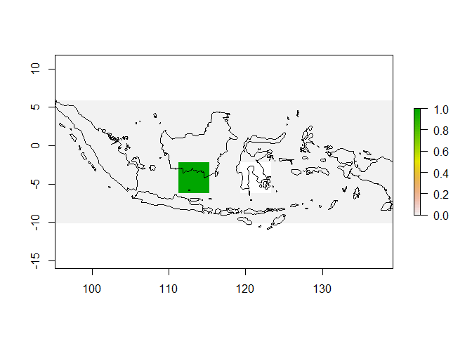
r[]<-v
{plot(r)
plot(d.indo,add=T)}
Neighbors values with spdep package
#neighbor list
nb<-cell2nb(nrow=nrow(r),ncol=ncol(r),type="queen")
#spatial weights matrix
nb.w<-nb2listw(nb,style="W", zero.policy=T)
#lagged values
v<-lag.listw(nb.w,values(r),zero.policy=F,NAOK=T)
## Warning in lag.listw(nb.w, values(r), zero.policy = F, NAOK = T): NAs in lagged
## values
##new raster
nb.r<-r
nb.r[]<-v
nb.r[]
##  [1] 0.000 0.000 0.000 0.000 0.000 0.000 0.000 0.000 0.000 0.000 0.000 0.000
## [13] 0.000 0.000 0.125 0.125    NA    NA    NA 0.000 0.000 0.000 0.000 0.000
## [25] 0.000 0.125 0.000    NA 0.000    NA 0.000 0.000 0.000 0.000 0.000 0.000
## [37] 0.200 0.200    NA    NA    NA 0.000 0.000 0.000
sum(nb.r[],na.rm=T)
## [1] 0.775
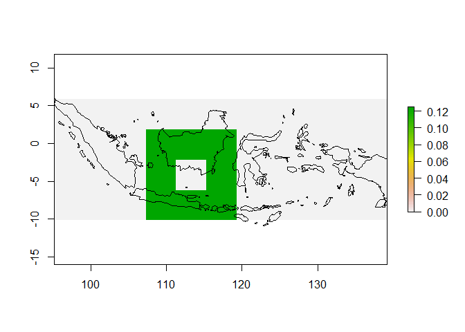
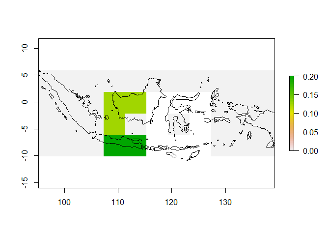
{plot(nb.r)
  plot(d.indo,add=T)}
 The output
raster shows higher values at the edges.
The output
raster shows higher values at the edges. nb2listw does not account for
the missing values at the edge of a raster.
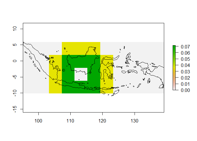
Neighbors values with raster package
#neighbor matrix
nb.w<-matrix(c(1,1,1,1,0,1,1,1,1),ncol=3)
#weights function
mean.W.style<-function(x){sum(x,na.rm=T)/(ncell(nb.w)-1)}
#new raster
nb.r<-focal(r,nb.w,pad=T,NAonly=F,fun=mean.W.style)
nb.r[]
##  [1] 0.000 0.000 0.000 0.000 0.000 0.000 0.000 0.000 0.000 0.000 0.000 0.000
## [13] 0.000 0.000 0.125 0.125 0.125 0.000 0.000 0.000 0.000 0.000 0.000 0.000
## [25] 0.000 0.125 0.000 0.125 0.000 0.000 0.000 0.000 0.000 0.000 0.000 0.000
## [37] 0.125 0.125 0.125 0.000 0.000 0.000 0.000 0.000
sum(nb.r[],na.rm=T)
## [1] 1
{plot(nb.r)
  plot(d.indo,add=T)}
Multi-lag neighbor matrix
For more ideas and exmpales see the OSGEO-GRASS application documentation of r.neighbors here.
#neigbor matrix
nb.w<-matrix(ncol=5,nrow=5)
nb.w[]<-0.5
nb.w[3,3]<-0
nb.w[1,1]<-0
nb.w[5,5]<-0
nb.w[5,1]<-0
nb.w[1,5]<-0
nb.w[2,2]<-1
nb.w[2,3]<-1
nb.w[2,4]<-1
nb.w[3,2]<-1
nb.w[3,4]<-1
nb.w[4,2]<-1
nb.w[4,3]<-1
nb.w[4,4]<-1
nb.w[]<-nb.w/sum(nb.w)
sum(nb.w)
## [1] 1
nb.w
##            [,1]       [,2]       [,3]       [,4]       [,5]
## [1,] 0.00000000 0.03571429 0.03571429 0.03571429 0.00000000
## [2,] 0.03571429 0.07142857 0.07142857 0.07142857 0.03571429
## [3,] 0.03571429 0.07142857 0.00000000 0.07142857 0.03571429
## [4,] 0.03571429 0.07142857 0.07142857 0.07142857 0.03571429
## [5,] 0.00000000 0.03571429 0.03571429 0.03571429 0.00000000
#weights function
mean.W.style<-function(x){sum(x,na.rm=T)/(length(nb.w[nb.w>0])-1)}
#new raster
nb.r<-focal(r,nb.w,pad=T,NAonly=F,fun=sum,na.rm=T)
nb.r[]
##  [1] 0.00000000 0.00000000 0.00000000 0.03571429 0.03571429 0.03571429
##  [7] 0.00000000 0.00000000 0.00000000 0.00000000 0.00000000 0.00000000
## [13] 0.00000000 0.03571429 0.07142857 0.07142857 0.07142857 0.03571429
## [19] 0.00000000 0.00000000 0.00000000 0.00000000 0.00000000 0.00000000
## [25] 0.03571429 0.07142857 0.00000000 0.07142857 0.03571429 0.00000000
## [31] 0.00000000 0.00000000 0.00000000 0.00000000 0.00000000 0.03571429
## [37] 0.07142857 0.07142857 0.07142857 0.03571429 0.00000000 0.00000000
## [43] 0.00000000 0.00000000
sum(nb.r[],na.rm=T)+sum(nb.r[1,])
## [1] 1
{plot(nb.r)
  plot(d.indo,add=T)}