Code: Nightlight statistics for spatial units
This is an easy and fast way to process DMSP-OLS nightlight data and to build your statistics, such as mean, min, max, or other. The script uses the GDAL python-based libraries. To install GDAL, visit the homepage here. See this guide on how to download and prepare the DSMP-OLS nightlight data. Here I build yearly nightlight statistics for all Chinese cities (Admin 2 level) using the spatial boundaries from DIVA-GIS.
Setup
library(raster)
library(clipr)
library(rgdal)
library(rgeos)
library(dplyr)
t<-tempfile()
Download administrative boundaries
if (!file.exists(file.path("data","CHN_adm2.shp"))){
  download.file("http://biogeo.ucdavis.edu/data/diva/adm/CHN_adm.zip",t)
  # unzip(t,list=T)
  x<-unzip(t,list=T)$Name
  x<-x[grep("CHN_adm2",x)]
  unzip(t,files=x,exdir="data",overwrite=T)
}
# list.files("data")
Rasterize shapefile
The nightlight DMSP-OLS version has a resolution of 0.00833 degrees (~1
km at the equator). That means for the extent of china the raster has
“only” xxx cells, which can still be coerced into a data frame without
crossing the vector size limit of your computer. Therefore, I would
always rasterize the administrative units (with the raster definition of
the nightlight) and then combine the data. The rasterize function of
the rgdal packages is slow and prone to errors, I, therefore,
recommend using gdal, which is a very fast way to
process raster data. This means that the R script “merely” produces
command lines that are sent to the system or pasted manually to the
terminal.
#loading Chinese boundaries
d<-readOGR("data",'CHN_adm2',stringsAsFactors=F,verbose=F)
d$ID_2<-as.integer(d$ID_2)
d.china<-d
#load one nightlight raster
r<-raster("data/F152007.tif")
#check if the layer and the raster have the same CRS
crs(d.china)
## CRS arguments: +proj=longlat +datum=WGS84 +no_defs
crs(r)
## CRS arguments: +proj=longlat +datum=WGS84 +no_defs
#crop nightlight raster to china's extent
r<-crop(r, d.china)
#slow rastarization with the raster package - and often encounters some error
# rr<-rasterize(d.china,r,field="ID_2",filename=file.path("r.china.cities.tif"))
#quick rasterization wiht gdal
cmd<-paste0(
  c(
    "gdal_rasterize",
    "-a ID_2",
    paste(c("-te",extent(r)[c(1,3,2,4)]),collapse=" "),
    paste(c("-tr",res(r)),collapse=" "),
    file.path("data",'CHN_adm2.shp'),
    file.path("data","r.china.cities.tif")
  ),
  collapse=" "
)
cmd
## [1] "gdal_rasterize -a ID_2 -te 73.5541656518887 18.1625002268218 134.770832073638 53.5625000851459 -tr 0.0083333332999931 0.00833333329998213 data/CHN_adm2.shp data/r.china.cities.tif"
system.time(
  system(cmd) ##run the command from within R
)
##    user  system elapsed
##    0.00    0.00    2.08
#laod new raster
r<-raster("data/r.china.cities.tif")
#test number of id values
length(unique(r[]))-1 # not counting zero values
## [1] 344
length(unique(d.china$ID_2))
## [1] 344
##save
r.china<-r
Note: It could be that your spatial units are too small to be captured by a nightlight pixel. The rasterization process intersects cell centroids with the spatial layer. Some small units might not touch any centroid and are lost while rasterizing. If you need those units in your analysis, I recommend building nightlight values from cells that touch the small polygon. I do not include the coded solution here, but you can write me an email if you encounter this problem.
Also note that you should avoid setting ‘255’ as the null value in the GDAL rasterization. Although this might ease the visualization in QGIS it conflicts with the data - ‘255’ is the ID_2 value of a city. Without setting the null value explicly, the raster uses zeros for cells outside the Chinese layer.
Crop nightlight raster to the china extent
flist<-list.files("data","F.*\\.tif$")
a<-lapply(
  flist,
  function(f){
    # print(f)
    r<-raster(file.path("data",f))
    r<-raster::crop(r,r.china)
    return(r)
  }
)
names(a)<-sub("\\.tif","",flist)
r.nl.stack<-a
Combine raster cell data
#china ids
d<-data.frame(
  ID_2 = r.china[]
)
#nightlight values
for (x in names(r.nl.stack)){
  # print(x)
  d[,x]<-values(r.nl.stack[[x]])
}
#exclude non-china areas
i<-which(d$ID_2==0)
d<-d[-i,]
#save
d.pixel<-d
Model DMSP data versions
Due to a change in the use of satellites over time, the nightlight data sometimes has several versions for one year, for example, F152007.tif and F162007.tif. You can either choose the most appropriate version for your analysis or pool both sources. The code here uses the average if there are two versions in one year.
d<-d.pixel
for (y in 2007:2008){
  # y<-2007
  i<-grep(y,names(d))
  # print(names(d)[i])
  if (length(i)>1){
    d[,paste0("dmsp.",y)]<-rowMeans(d[,i])
  } else {
    d[,paste0("dmsp.",y)]<-d[,i]
  }

}
d.dmsp.modeled<-d
names(d)
## [1] "ID_2" "F152007" "F162007" "F162008" "dmsp.2007" "dmsp.2008"
Collapse to spatial unit level
Depending on your study area and research question, you can create your statistics. Here I only calculate the mean, median and sum of yearly nightlight within each Chinese city.
d<-d.dmsp.modeled
d<- data.frame(
  d %>%
    group_by(ID_2) %>%
    summarise_at(
      .vars = paste0("dmsp.",2007:2008),
      .funs = c(
        mean="mean",
        median="median",
        sum = "sum"
      )
    )
)
#save
d<-d[order(d$ID_2),]
d.collapse<-d
write.csv(d,"chinese.nightlight.csv",row.names=F)
names(d)
## [1] "ID_2"             "dmsp.2007_mean"   "dmsp.2008_mean"   "dmsp.2007_median"
## [5] "dmsp.2008_median" "dmsp.2007_sum"    "dmsp.2008_sum"
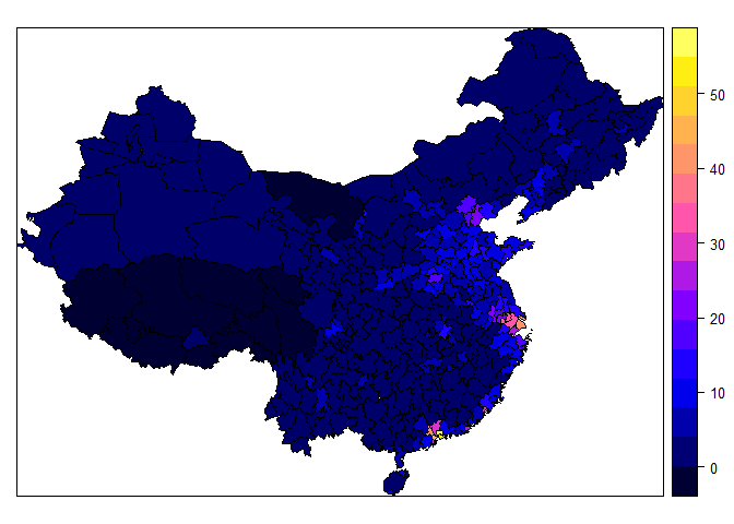
Plot Chinese nightlight data
#read nightlight data
d<-read.csv("data/nightlight-dmsp-statistics.csv")
#read shapefile
ch<-readOGR('data','CHN_adm2',verbose=F)
#simplify geometry
ch2<-gSimplify(ch,0.05)
ch<-SpatialPolygonsDataFrame(ch2, data=ch@data)
##merge with nightlight data
ch<-merge(ch,d,by="ID_2",all.x=T)
#plot
jpeg("nightlight-dmsp-statistics.jpeg")
spplot(ch,zcol="dmsp.2008_mean")
dev.off()
## png
##   2
spplot(ch,zcol="dmsp.2008_mean")